

Continuing our series — see here for Part 1, and Part 2 — let’s look at Makin and Orban de Xivry’s Statistical Mistake #4: Spurious Correlations.
This one is easy to understand, though nonetheless common. The authors refer to situations like the one illustrated in their Figure 2, shown below, in which the correlation calculated between two variables is driven solely by a few, or even one, data points. In other words, the correlation coefficient doesn’t really represent the relationship among the data.

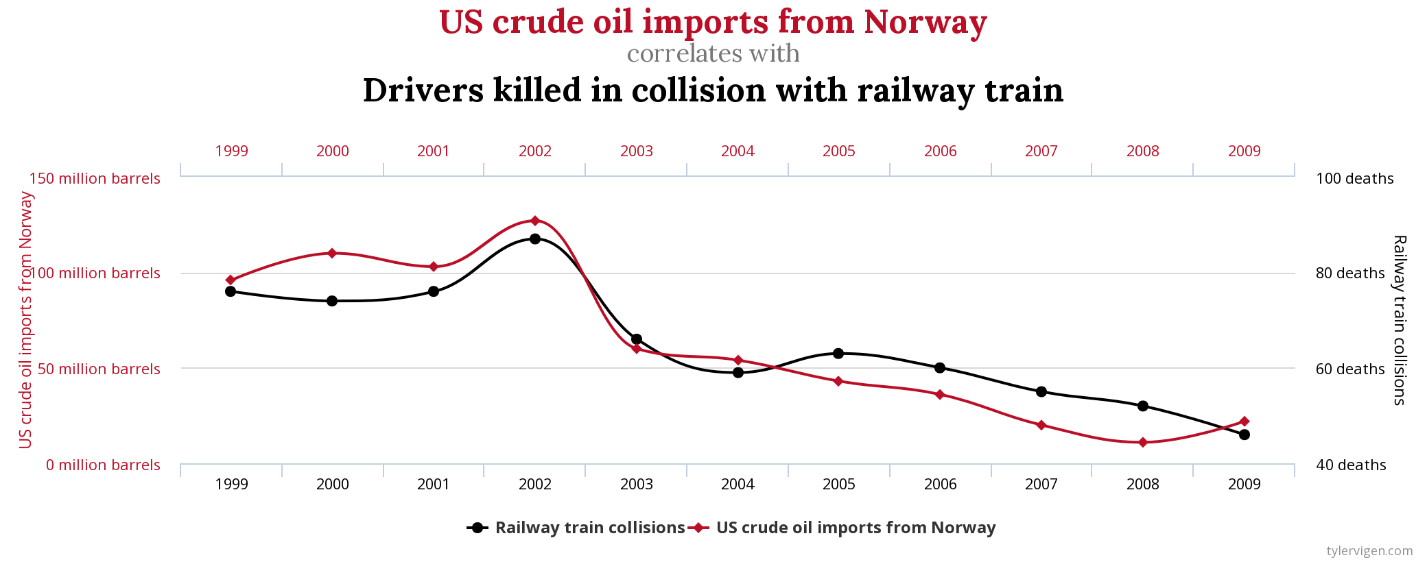
I’d call this “non-robust” rather than “spurious” — I associate spurious correlations with relationships that are entirely coincidental — but I don’t know if there’s a real definition of the term. When I hear “spurious correlations,” the first thing that pops to mind is a wonderful collection with that name of true, but absurd, correlations like this one (r=0.9545):
In any case, the point is that one should be wary of correlation values that rely on a small fraction of the data. Equivalently, one should be aware that simply calculating a correlation coefficient doesn’t in any way guard against this mistake.
Makin and Orban de Xivry note that there’s not necessarily anything wrong with the far-out points — they may be perfectly valid observations and not “outliers” to be removed. I was reminded of this general issue when discussing the classic Luria-Delbrück experiment in my biophysics class this week, in which rare data points far from the mean are the “smoking gun” of spontaneous mutations driving selection in a population. The “mistake” of spurious correlations arises not from the data, but from the meaning one assigns to a correlation coefficient, which is just a particular way of characterizing the data.
There are two solutions to this problem. One is to use more robust assessments of correlations, some of which are listed in the article. The more important, and even simpler, solution is to plot your data. This seems obvious, and thankfully it is quite common throughout the natural sciences. Seeing the spatial arrangement of the points lets us grasp their relationship much better than seeing an r value. I’ve been surprised, however, to routinely see lists of correlation coefficients, with no graphs to be found, in papers in economics and other social sciences.
I don’t have a lot to say about this mistake. The solution of plotting things is a powerful and general one. Of course, making plots doesn’t stop people from irresponsible analyses, but at least it makes the flaws more evident.
Not long ago I learned that “regression discontinuity analysis” is a thing — separately fitting curves to either side of some datapoint to infer the magnitude of a step that occurs at that point. In principle this is fine; in practice, noise will make it ripe for overfitting, in a way that is reminiscent of these spurious correlations. See here for an example. Again, plotting makes the flaws clear.
Discussion topic: What are we trying to convey when stating a (Pearson) correlation coefficient? Can one go “backwards” frorm an r value to an accurate picture of what the data look like?
Exercises: I couldn’t come up with any non-boring simulation exercises. I sketched one in which we generate a handful of datapoints of the form y = 1 – x + noise with x between 0 and 1, toss in another datapoint at (1, y_outlier), and plot the resulting r vs y_outlier. It’s not that exciting, however.
Exercise 4.1 Come up with a good simulation exercise related to this point. (Maybe see above.)
Exercise 4.2 Find examples of non-robust correlations in papers. It has definitely come up in our journal club, but I’ve neglected to make notes of when.
I warned you that some of these posts would be rather minimal!
Today’s illustration…
Yet another attempt at waves on a shore. I still can’t the foam to look decent, but at least this time there are turtles!
— Raghuveer Parthasarathy, October 22, 2020
