
 NOTE: This will only be of interest to a subset of the very small number of people who calculate things related to two dimensional viscosity. For the rest of you, here’s a link to the previous post, on witchcraft!
SYNOPSIS: I describe and provide MATLAB code (here) to calculate the hydrodynamic drag and diffusion coefficients for the translational and rotational motion of an object in a two dimensional membrane, implementing the set of series equations in Hughes, Pailthorpe, and White’s classic 1981 paper [1], and correcting an error therein.
Membrane drag: background
The diffusion coefficient (D) of an object in a fluid is determined by the temperature (T) and the object’s hydrodynamic drag (b), as Albert Einstein, Marian Smoluchowski, and William Sutherland all realized in the first few years of the twentieth century; specifically, D = k T / b, where k is Boltzmann’s constant. For a sphere in a three dimensional liquid, like water, b is a simple function of the sphere’s radius (R) and the liquid viscosity (η): b = 6 π η R. For an object in a two-dimensional liquid, the hydrodynamic problem becomes much more difficult. In fact, for an isolated 2D liquid, there is no well-defined drag coefficient, a result known as Stokes’ Paradox.
For a 2D liquid embedded in a 3D liquid, however, such as a cellular membrane in water, flows are well-behaved and there is a robust drag coefficient. In a landmark 1975 paper, Saffman and Delbrück derived the solution to the problem of 2D diffusion, but only in the limit of very large membrane viscosity [2]. In 1981, Hughes, Pailthorpe, and White (HPW) solved the general case, providing both a set of integrals that can be numerically integrated to give the rotational and translational drag coefficients, and a set of equivalent infinite series expressions. In addition, they wrote asymptotic expressions that are valid for large membrane viscosity, and that reduce to the Saffman-Delbrück equations in the appropriate limit.
Implementing the HPW series equations
My lab has been examining membrane diffusion for several years (e.g. [3], [4], [5]; this post). We’ve made use of the HPW asymptotic expressions and also the integral equations; the latter are slow to calculate and a bit tricky to implement. Using them “involves substantial computational efforts” [6], which has led one group to employ various ad-hoc approximations [6].
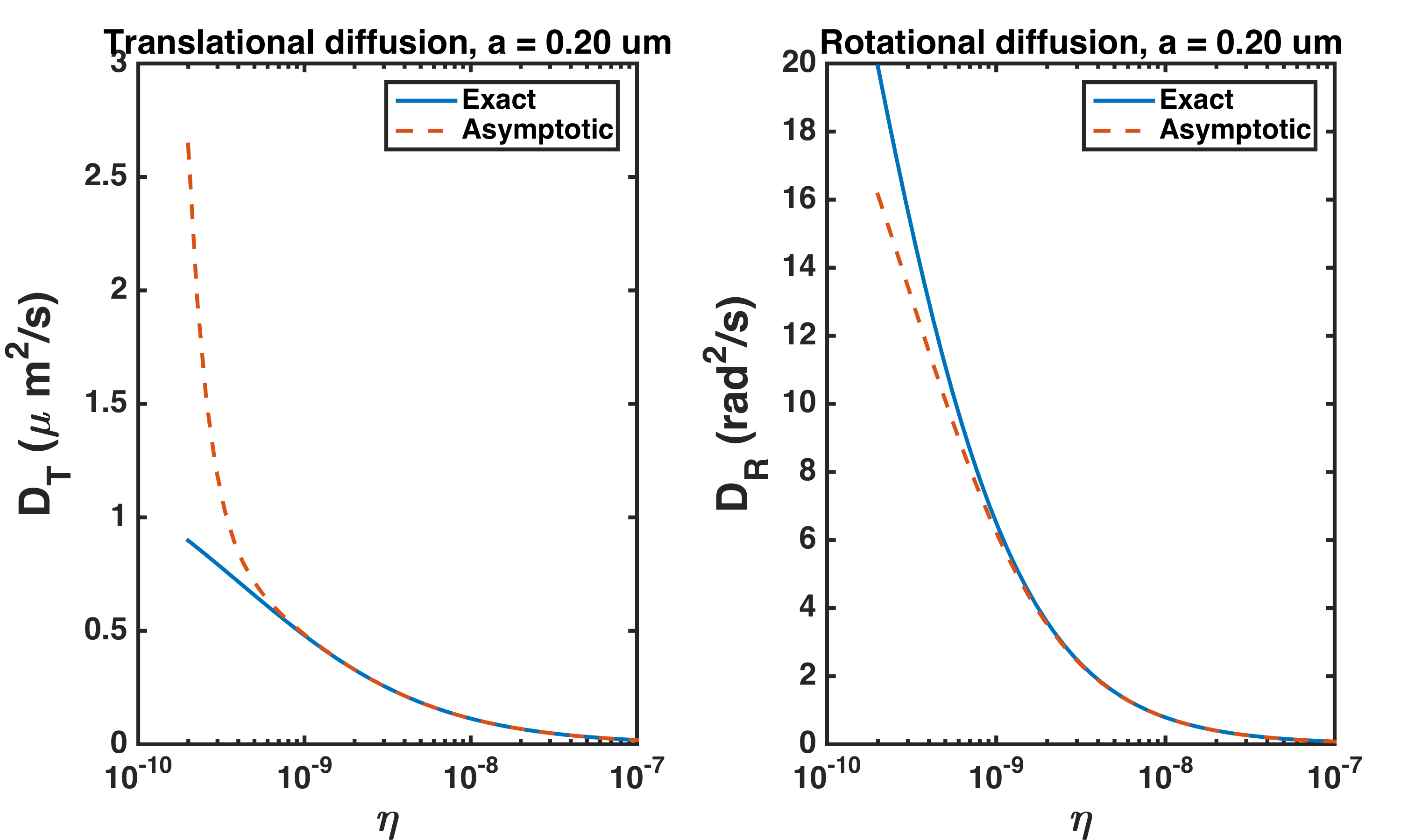
HPW’s infinite series expressions are elegant, but rather daunting. A few years ago, I tried to implement them and failed. A week or so ago, I revisited this, and in the process of examining each piece of solution, I realized that there is an error (a typo, presumably) in one of the HPW equations. (I’ll describe this a bit more below.) I guessed the fix, and was then able to write a simple MATLAB function that encodes the series solution. It is very fast, and agrees with the asymptotic expressions in the appropriate limit (see graph, below). (See Update #2 at the end, however, about problems for ε > 1.)
Available Code: My MATLAB function HPW_drag.m is available in this public Git repository, https://github.com/rplab/HPW_MembraneDiffusion. It calculates the translational and rotational drag and diffusion coefficients, given input viscosities and the inclusion radius.
Also in the repository is a function for calculating the best-fit membrane viscosity and inclusion radius, given (measured) rotational and translational diffusion coefficients: HPW_fit.m.
If you find the functions useful, let me know!
The fix
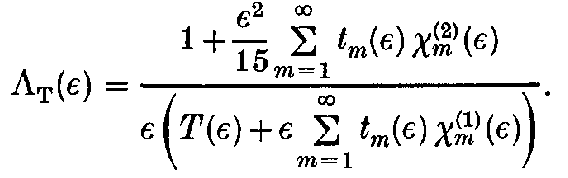
In case anyone wants the details, and a mathematical challenge: There are lots of pieces that make up the HPW equation for the translational drag coefficient, written here in a nondimensional form Λ:

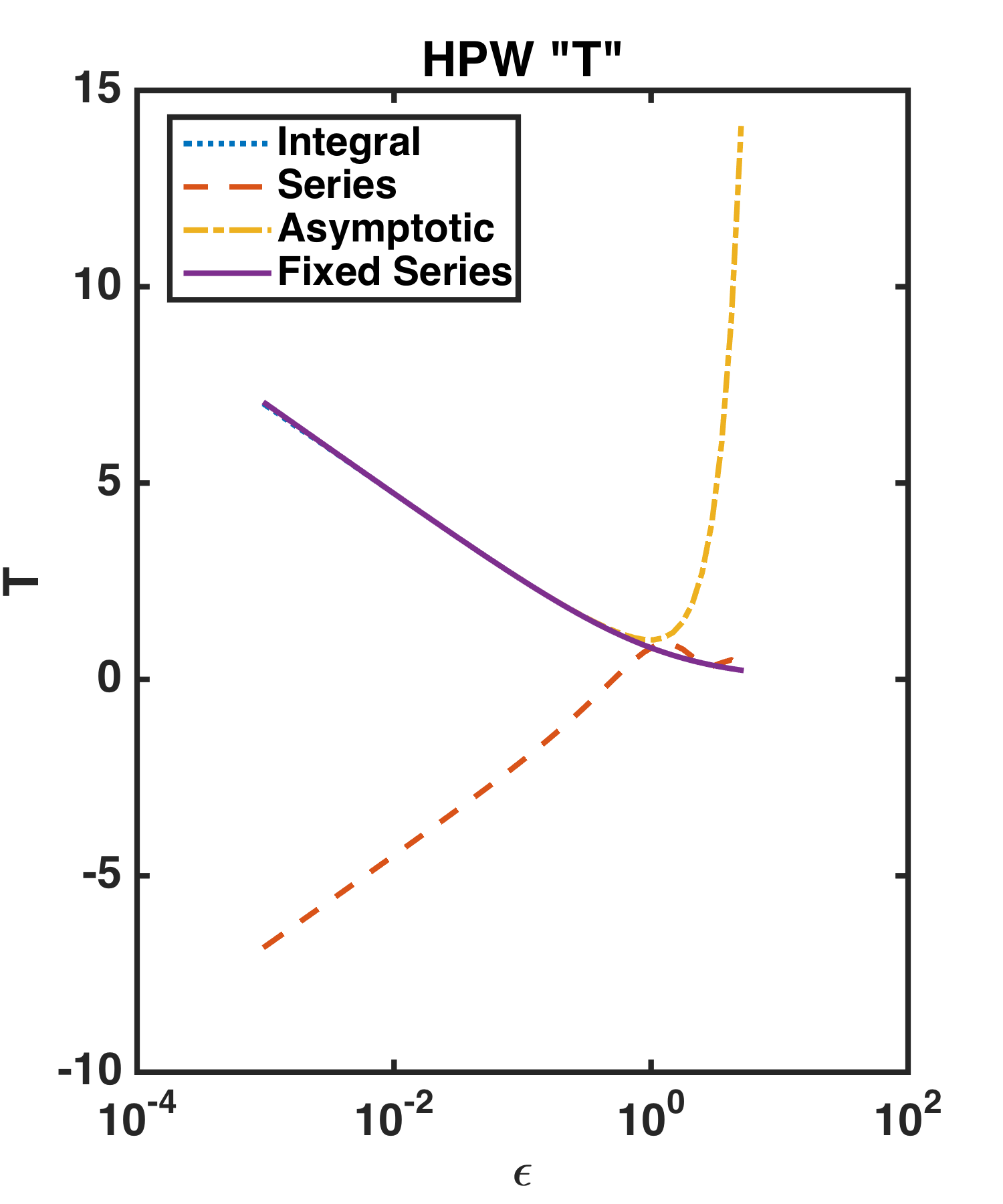
I realized that one of them, the function T(ε), wasn’t behaving as it should. Here’s T(ε) from the integrals, from the asymptotic expressions, and from the series equations (A11-A13 in the paper):

T(ε) is written in two parts:

After trying various things and staring a lot, I guessed that the “ln(2ε)” should be ln(2/ε). This works! The results are sensible, and in agreement with the integral solution and the asymptotic expression.
But, you might be gasping, I didn’t actually solve the equations to figure out and fix the error! You’re right! If you’d like to give it a shot, the relevant thing to do is to take the Mellin transform of

which gives:

Then, “closing the inversion contour to the left and evaluating the residues at the poles of the integrand, we obtain…” Eq. A11-A13, above. However, it’s been 20 years since I’ve done a contour integral, so I’m going to leave this as an exercise for the reader!
UPDATE #1:Tatiana Kuriabova at Cal Poly verified my guess for the correct Eq. A13, and graciously shared a derivation! You should be able to click this link, “kuriabova_hpw_eqa13“, and there should also be a “Download” button at the bottom of this post.
UPDATE #2: Eugene Petrov at LMU Munich sent a very helpful email pointing out that my series solution has severe problems converging for ε near 3, and ε > 10, similar to issues he ran into years ago when working on [6]. Embarrassingly, this ε range is just beyond what I tested! Below, I show D_T vs. 2D viscosity extending a bit further to lower viscosity; the bad behavior is clear. Interestingly, this doesn’t involve problems with the “T” term (Eq. 13), but other infinite series in the HPW calculations. Petrov further suggests that there are additional typos in the 1981 paper. Thankfully, if one cares about very low viscosity / small object radius / high ε, the convergence issues are obvious immediately upon running the series script in this range; if one cares about higher viscosity / larger objects / lower ε, as has been the case in my lab, the series works well.

UPDATE #3 (Aug. 20, 2021): Earlier this year, I realized that (i) a lot of the gamma function calculations in the various infinite series could be simplified, and (ii) the issues with series solution divergences for ε near 3.45 (and other values) can be glossed over with the following approach:
The dimensionless translational drag is given by HPW Eq. 3.68:
We can write this as:

Our troubles arise because N(ε) and D(ε) go to zero at ε ≈ 3.44 (and elsewhere), but not quite at the same ε due to numerical issues. Simply setting N/D = 1 is a fairly good approximation for Λ(ε), but even better is to write a polynomial approximation:
N(ε) / D(ε) ≈ c0 + c1 log(ε) + c2 log(ε)2:

Quite good! The GitHub code now incorporates both of these changes.
References
[1] B. D. Hughes, B. A. Pailthorpe, White L. R., The translational and rotational drag on a cylinder moving in a membrane. J Fluid Mech. 110, 349–372 (1981). Note: this paper can be hard to obtain, so here’s a link to a PDF.
[2] P. G. Saffman, M. Delbrück, Brownian motion in biological membranes. Proc Natl Acad Sci USA. 72, 3111–3113 (1975)
[3] T. T. Hormel, S. Q. Kurihara, M. K. Brennan, M. C. Wozniak, R. Parthasarathy, Measuring Lipid Membrane Viscosity Using Rotational and Translational Probe Diffusion. Phys. Rev. Lett. 112, 188101 (2014).
[4] T. T. Hormel, M. A. Reyer, R. Parthasarathy, Two-Point Microrheology of Phase-Separated Domains in Lipid Bilayers. Biophys. J. 109, 732–736 (2015).
[5] V. L. Thoms, T. T. Hormel, M. A. Reyer, R. Parthasarathy, Tension Independence of Lipid Diffusion and Membrane Viscosity. Langmuir. 33, 12510–12515 (2017).
[6] E. P. Petrov, P. Schwille, Translational diffusion in lipid membranes beyond the Saffman-Delbruck approximation. Biophys J. 94, L41–L3 (2008).
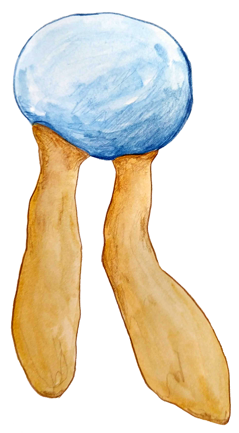
Today’s illustration
A lipid. How many lipids have I drawn? Dozens, easily. A hundred?
— Raghuveer Parthasarathy. September 3, 2018
