
(A more technical post than most, in which we look at bacterial population densities, and watch a movie.)
 This term I taught a graduate biophysics course, about which I’ll write a recap later. Bacteria came up a lot in the course, both because they’re important but also because they offer many nice illustrations of how physical principles of diffusion, hydrodynamics, and stochasticity govern how life works. A benefit of teaching a graduate course is that I learn things, too! I’ll describe here something about chemotaxis that I wasn’t previously aware of.
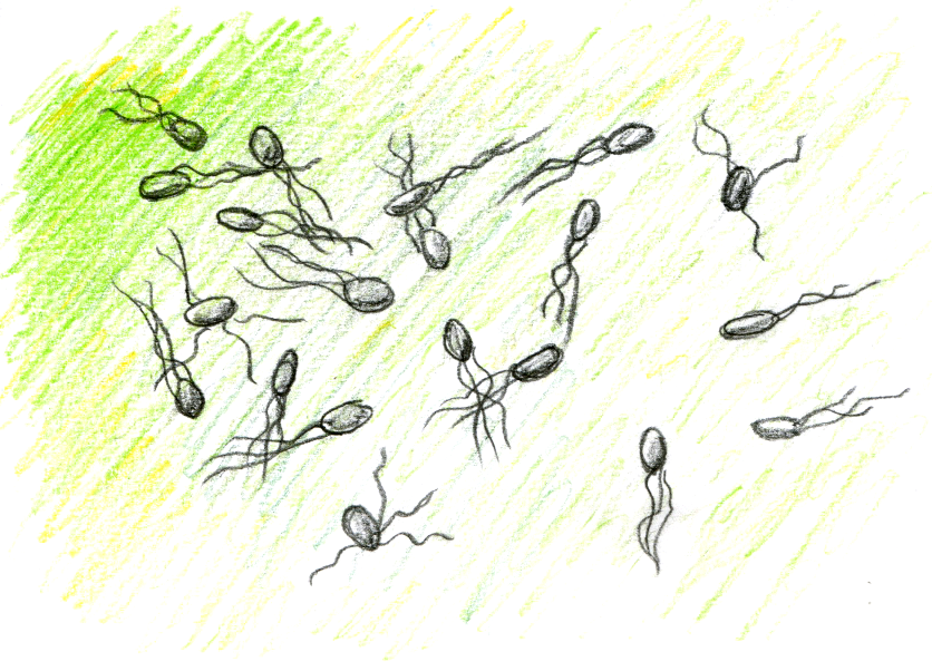
Motile bacteria will migrate towards higher concentrations of attractants (e.g. nutrients). Bacteria like E. coli move in a sequence of roughly straight-line, constant velocity “runs”…
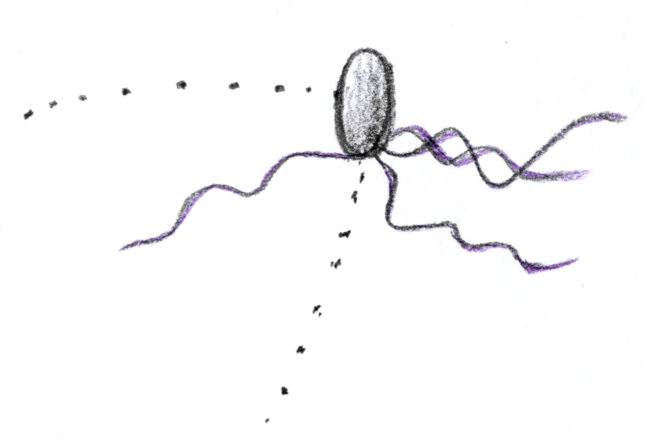
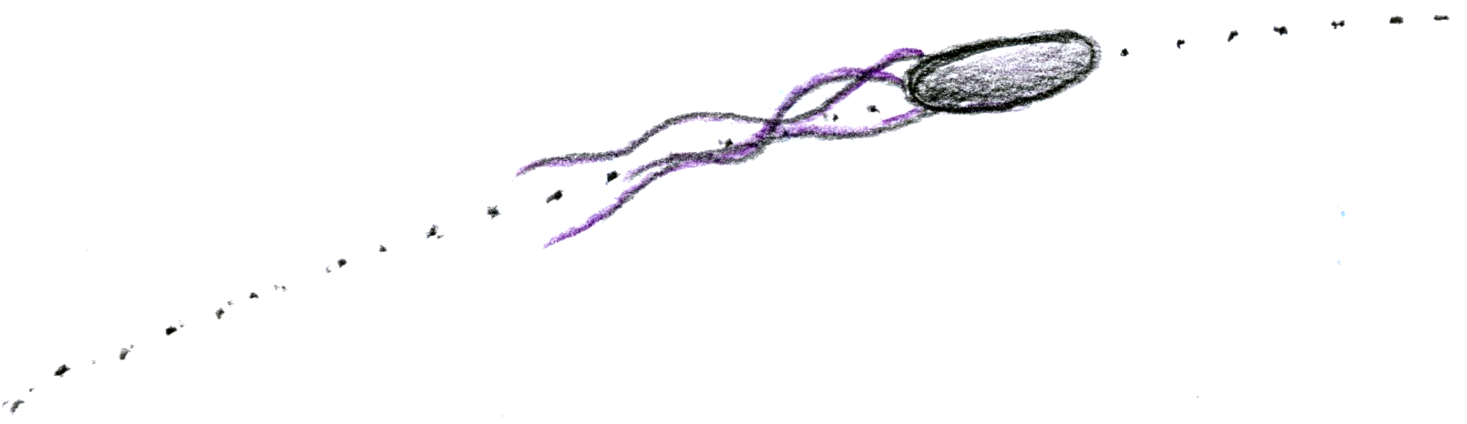 … separated by “tumbles” at which they randomize their direction:
 If the bacterium senses that the nutrient concentration is increasing with time, the probability per unit time of tumbling decreases (and so, on average, the run length increases). In other words, if the bacterium is moving in a “good” direction, it’s more likely to continue in that direction. All this well known, nicely described, for example in Howard Berg’s classic book, which I first read at least a decade ago (2000?).
The new (to me) part: Given a bunch of bacteria, it’s clear that the process described above will increase the bacterial concentration at regions of high attractant concentration. But how much? If I double the attractant concentration (c) in one area compared to another, does the bacterial population density (P) double? What is the relationship between c and P?
Remarkably, in retrospect, I had never thought about this question, and had never stumbled upon a discussion of it, until seeing it as an exercise in Bill Bialek’s recent book. As Bialek sketches, one can write a simple model of this process in which we state that the tumble rate (r) is a linear function of ∂c/∂t, the perceived rate of change of the concentration. Just given this, we can derive, analytically, the form of the steady-state bacterial concentration P(c(x)). (We consider just one dimension, x; I expect that the answer easily generalizes to higher dimensions.) I elaborated slightly and assigned this as a homework problem for my class. (If you’re interested, it’s #5 of this: Homework5: the original by Bialek is #49 of this: fromBialek_page154.)
The answer is amazing:
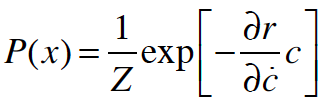 where Z is some normalization. In other words, the bacterial density follows a Boltzmann distribution, analogous to P = exp(-Energy/Temperature), with the local concentration playing the role of energy. The analog to the temperature in statistical mechanics is the proportionality between the tumble probability and ∂c/∂t. (I don’t think I can write a c with a dot on it here…)
It’s such a nice, succinct result! If we double the nutrient concentration, we increase the bacterial density by a factor of e^2 = 7.4.
In retrospect, I should perhaps not have been surprised, since:
- the concentration gradient changes the likelihood that a right-moving bacterium becomes a left-moving one, or vice versa, and so is reminiscent of forward and backward reaction rates in chemical reactions, the equilibrium concentrations of which are given by a Boltzmann expression dependent on the free energy.
- it seems that every distribution in nature is exponential, Gaussian, or Poisson, so we had a 1/3 chance of finding a Boltzmann distribution!
One can derive the above result analytically with some careful thinking and a bit of time. One can also simulate this chemotaxis model and validate the result with less thinking and more time. I didn’t assign the simulation to my students (though they had several other programming assignments), but I’ve done it myself for kicks.
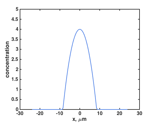
Consider, for example, this parabolic concentration profile:
 Let’s watch 200 bacteria moving (in 1D), responding to this c(x) as in the Bialek model, i.e. with a tumble rate that is linearly dependent on the perceived rate of change of c:
The movie is fun, but it’s clearer to look at the histogram of bacterial number, i.e. P(x), which the theory would predict is a Gaussian. It is, with the proper width and shape predicted by the model. The plot on the left shows the final (steady-state) P(x) together with exp(-beta c(x)), where beta = ∂r/∂\dot{c} and the plot on the right shows the evolution of P(x) with time.
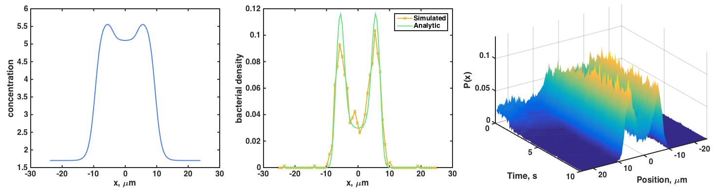
 We can make weirder concentration profiles, and again find that the simulated P(x) agrees with the analytic P(x) = exp(-beta c(x)):
 My MATLAB code for the simulation, which contains descriptions of the parameters, is here. (Note: there’s considerable room for improvement — take this as a sketch!)
What’s the moral of this story? Yet again, it shows us that random processes can be described by simple rules. It also gives us a simple way to potentially link observed bacterial spatial distributions with underlying chemical gradients, which we’re presently applying in the lab to some of our bacterial imaging experiments.
