Three views of a statistics puzzle

On his blog today, Andrew Gelman posted a simple to state, clearly realistic, and surprisingly deep statistics puzzle sent to him by Ariel Rubinstein and Michele Piccione, from their paper, “Real People Aggregating Signals: An Experiment and a Short Story” Article Link:

A very small proportion of the newborns in a certain country have a specific genetic trait. Two screening tests, A and B, have been introduced for all newborns to identify this trait. However, the tests are not precise. A study has found that: 70% of the newborns who are found to be positive according to test A have the genetic trait (and conversely 30% do not). 20% of the newborns who are found to be positive according to test B have the genetic trait (and conversely 80% do not). The study has also found that when a newborn has the genetic trait, a positive result in one test does not affect the likelihood of a positive result in the other. Likewise, when a newborn does not have the genetic trait, a positive result in one test does not affect the likelihood of a positive result in the other. Suppose that a newborn is found to be positive according to both tests. What is your estimate of the likelihood (in %) that this newborn has the genetic trait?

Because the puzzle will be discussed tomorrow, I thought I’d note down my thoughts (hoping that they’re correct) now. This is, therefore, a hastily written post! I’m going to be very sloppy about elaboration and notation; hopefully, if you’re interested, you can follow along. It’s also possible I’m wrong, but I’m willing to risk embarrassment… Also, I’m not proofreading this. Beware!

I found this a fun and puzzling problem for two reasons: (1) It’s not immediately obvious why we don’t need the false positive and false negative rates for the tests, and (2) Simulating it is more challenging than it initially seems!

Before reading on, I strongly recommend thinking about the puzzle. What’s your answer?

… [pause] …

I solved the problem with algebra, which just takes a few lines, then I simulated it, which took me much longer, and then I came up with a mediocre and unsatisfying “intuitive” explanation. In reverse order:

An intuitive, approximate explanation

Suppose we only had Test A, and we want to know what the probability of the newborn having the genetic trait is, given a positive result for Test A. It’s 70%, as stated in the question. The end.

We actually have Test A and Test B, however. It’s tempting to think the following: The probability of having the trait is 1 minus the probability of not having the trait given Test A’s information and not having the trait given Test B’s information, and is therefore 1 – 0.3×0.8 = 0.76, i.e. 76%. This is wrong, however: it doesn’t account for the probability of two positive results being greater if the trait is actually present. Instead of multiplying by 0.8 to incorporate the information from the second test, we should multiply by something like p x 0.8 where p is the overall proportion of newborns with the trait. (If this sounds unsatisfying, I agree…) Therefore, the answer is something like 1 – px0.3×0.8. For p = 1.0%, for example, the probability of the newborn having the trait is (roughly) 0.9976. This isn’t correct, but is closer to the correct answer than 0.76 (see below).

Simulation

Simulating questions of statistics and probability is often a great way to get insights or answers, bypassing algebraic exactness. (That’s a flaw or a virtue, depending on your perspective.) I thought this would be simple to simulate, but I found it challenging for a reason that highlights one of the interesting aspects of the problem.

We can imagine a population of N people, with probability p of having the trait. We then simulate the test results. We don’t know, however, for either test what the probability that someone with the trait tests positive is (the true positive rate) or the probability that someone without the trait tests positive (the false positive rate). How, then, can we model our population?

It seems like we have, for each test, two unknown parameters: the true and false positive rates. However, we also know the “flip side” of this: the probability that someone who tests positive has the trait, i.e. p(H | A), where H means “having the trait” and A means “positive for Test A.” This is 0.7. (And for B, p(H|B) = 0.2.) Therefore, we don’t really have two unknown parameters, just one, which we can fold into an overall probability for a positive test A (or B). By Bayes’ rule:

where p(H) (which I’ll also write as p below) is the probability in general of having the trait.

What’s p(A)? Who knows?! Let’s take the classic physics approach of making something up, and see if our result depends on its value! (For my favorite illustration of this, note the blog’s title.)

Here’s some Python code, without adequate explanation. Aside from setting parameters, it’s only about a dozen lines.

import numpy as np

N_trials = int(10)  # number of trials over which to average the results
N = int(1e6) # population size per trial
p = 1e-2 # frequency of the trait in the population

r = np.random.rand(N, N_trials) # a bunch of random numbers
rA1 = np.random.rand(N, N_trials) # a bunch of random numbers
rA2 = np.random.rand(N, N_trials) # a bunch of random numbers
rB1 = np.random.rand(N, N_trials) # a bunch of random numbers
rB2 = np.random.rand(N, N_trials) # a bunch of random numbers

has_trait = r < p # true if the person has the trait

# Things we know:
p_HA = 0.7 # probability that if test A is positive, the person has the trait
p_HB = 0.2 # probability that if test B is positive, the person has the trait

# Things we don't know and that I'm making up, constrained by the things we know!
# To simulate the test results, we need values for the true and false positive 
# rates, p(A|H) and p(A|~H). (And for Test B). 
# However, these must give the above p_HA (and p_HB), so we don't have 
# two parameters to make up, just one, which I can fold into an overall 
# probability for a positive test A (or B)
p_A = 0.01 # overall probability for a positive result on A
p_B = 0.001 # overall probability for a positive result on B
p_AH = p_HA*p_A / p # probability of a positive result on test A, for someone with the trait
p_BH = p_HB*p_B / p # probability of a positive result on test A, for someone with the trait
p_AnH = (1-p_HA)*p_A / (1-p) # probability of a positive result on test A, for someone without the trait
p_BnH = (1-p_HB)*p_B / (1-p) # probability of a positive result on test A, for someone without the trait

# the simulated test results, on the population
results_A = has_trait*(rA1 < p_AH) + ~has_trait*(rA2 < p_AnH)
results_B = has_trait*(rB1 < p_BH) + ~has_trait*(rB2 < p_BnH)

# the probability we care about: having the trait *and* being positive for A and B
p_final_eachTrial = np.sum(results_A*results_B*has_trait, axis=0) / np.sum(results_A*results_B, axis=0)

p_final = np.mean(p_final_eachTrial)
p_final_std = np.std(p_final_eachTrial)
print(f'Probability of having the trait: {p_final:.4f} +/- {p_final_std:.4f}')

What does it tell us?

p(H)	p(A)	p(B)	Probability of having the trait
1.0%	0.01	0.001	0.9821 +/- 0.0101
	0.003	0.01	0.9862 +/- 0.0034
	0.007	0.003	0.9851 +/- 0.0058
	0.003	0.007	0.9818 +/- 0.0071
	0.001	0.01	0.9836 +/- 0.0081

(If I had more time, I’d make graphs…)

As hoped, it looks like the probability of having the trait is independent of our choice of p(A) or p(B)! And, as we can see, this probability of having the trait is far greater than the naïve value (98.5% rather than 76%).

Algebra

Notation:

H = the newborn has the genetic trait.
~H = the newborn does not have the genetic trait.
A = Test A is positive
~A = Test A is negative
B = Test B is positive
~B = Test B is negative

We want to know P(H | A U B), i.e. the probability that the newborn has the genetic trait conditional on Test A and Test B being positive. From Bayes:

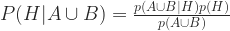
Bayes again:

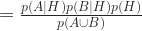
Now expand the denominator by enumerating all the terms that make it up:

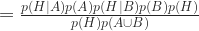
Combining these and doing a few lines of algebra that I don’t feel like typing from my scribbled notes:

We know all four numbers in the last fraction!

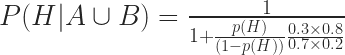
Therefore, for p(H) = 1%,

or 98.3%. Voila!

(If the frequency of the trait in the population is p(H) = 0.1%, the probability that our positive-testing newborn has the trait is 99.8%.)

Conclusions

This statistics problem is simple to state, and obviously relevant to real-world issues. I would hope that any doctor, epidemiologist, or public health practitioner could solve it, solve it quickly, and explain it better than me. In any case, it’s a fun puzzle, and though I neglected a fair amount of “real” work today to do it, I feel I’ve learned things! It’s remarkable that the addition of the superficially mediocre Test B adds so much to the tests’ interpretation.

Since this is a very quick post, I won’t elaborate much on a pointer to my pop-science biophysics book, though I’ll note that issues of predicting traits from tests comes up (in words, not math), touching on topics like giant chickens, human height, and genome sequencing.

Today’s illustration

Also extremely rapidly done, and fairly awful.