Muskrats, Arts and Crafts

How can we describe a population expanding into a new environment, like an invasive species spreading into virgin territory, or a disease infiltrating a community of susceptible hosts? Would the speed at which the population’s front advances be constant, like a car driving along a highway, so that if it travels 60 miles in one hour it will travel 120 miles in two? Or would it be sub-linear, like a diffusing gas, meandering in space so that it takes more than twice the time to cover twice the distance? Or would its distance-traveled be growing exponentially with time, if the organisms are constantly reproducing?

This is a classic question in ecology, and it maps onto classic physical models of reaction and diffusion. The topic came up during a journal club discussion of an elegant paper from Jeff Gore’s group:

S. R. Gandhi, E. A. Yurtsev, K. S. Korolev, J. Gore, “Range expansions transition from pulled to pushed waves as growth becomes more cooperative in an experimental microbial population.” PNAS, 113: 6922–6927 (2016).

In discussing the background to it, I told the story of muskrats invading Europe, since (i) it’s a beautiful and often-cited example of range expansion, (ii) it links clear data with compelling mathematical models, (iii) no one in the room, I think, was aware of it, and (iv) it’s muskrats invading Europe! Much of what I briefly discussed is in the book, “Diffusion and Ecological Problems: Modern Perspectives,” by Akira Okubo & Simon Levin. Here I’ll elaborate further, and also tackle re-plotting and analyzing some old data.

Enter the muskrat

Muskrats (pictured above) were suddenly and accidentally introduced to Europe in 1905, when five of them escaped from a farm in what is now the Czech Republic. The descendents of these five Bohemian pioneers spread across much of Europe, and they now number in the millions. Their spread was monitored, leading to this map of their range over time:

The graph is from a classic paper:

J. G. Skellam, Random Dispersal in Theoretical Populations. Biometrika. 38, 196–218 (1951)

(It’s also reprinted in Okubo and Levin.) On the right, I’ve overlaid this onto Google Maps’ view of the area.

To assess “distance vs. time” for the muskrats, we plot the square root of the area vs. time. The graph is again from Skellam:

We notice two striking things:

1. The relationship is linear. Like a car on a highway, distance is proportional to time.
2. The relationship is remarkably linear.

Data scraping, the new- and old-fashioned ways

Let’s first think about 2. Can we reproduce Skellam’s Figure 2? Unfortunately, the original data seems to be in an old German book that I can’t get my hands on:

Ulbrich, Johannes, “Die Bisamratte. Lebensweise, Gang ihre Ausbreitung in Europa, Wirtschaftliche Bedeutung und Bekampfung” (C. Heinrich, Dresden, 1930).

As the next best thing, can I reproduce Figure 2 from Figure 1? In other words, can I extract the range-area for each of the Muskrat curves? Why bother? First, to assess our trust of Figure 2, and second, to illustrate two points that I’ll hopefully come back to in another blog post, that we might learn things from re-plotting data from papers, and that this is in general not straightforward.

I will pause for a moment to let you, dear reader, think of at least two ways to do this — one modern way, and one that could have been done in 1951 (or 1851). When you’re done thinking scroll down…

A Modern Way

We’d like to get the area inside each of the contours. One way to determine this is to fill in the contours, and count how many filled pixels there are. First, we’ll need to (by hand) erase the year labels, and draw to fill in the gaps in the contours. Of course, this involves some extrapolation, since we’re making up data points that don’t exist. (Undoubtedly, the contours themselves are extrapolations from discrete observation sites.)

We could then “paint bucket” the regions, and count pixels. To be a bit more sophisticated, I instead did a watershed transformation of an images of the contour map — a common approach to identifying regions in images, analogous to treating intensity as topography and imagining what areas would get filled in by distinct basins if the landscape were to fill with water. Simply applied, this never works well; there are tricks one can apply to force minima onto the landscape at particular places, in this case at all pixels corresponding to an “eroded” version of the contour lines, that help. Doing this, one finds the following regions:

… from which it’s simple to make a map of the square root of the number of pixels vs. year. Here it is, with a best-fit line:

Just like Skellam showed, it’s remarkably linear! The fractional uncertainty in the sope is about 3%. (In case you want this in real units, there are about 1.4 px/mile.)

The Hand-crafted, Artisanal Way

How can one make this plot without recourse to modern, computer-based methods? Like this:

I printed out the map, cut it, and weighed the pieces of paper. Here’s the graph of distance (i.e. square root of mass) vs. time:

Again, remarkably linear! (The fractional uncertainty of the slope is again 3%.)

Which approach — digital or analog — is faster? Which is more fun? The answer to both is: the analog, paper-weighing, arts-and-crafts approach.

Muskrat waves

Why is it that the muskrat dispersal has a well-defined, constant velocity? Is this some specific consequence of muskrat biology, or a more general feature of populations? There are two key things that these animals are doing: (i) moving, and (ii) reproducing. Let’s think of their motion as a random walk, at least from one generation to the next — the children of adult muskrats are (aside from the pressures of competition) as likely to go north, south, east, or west from their home. A random walk, whether of a gas molecule or an aimless bacterium, can be characterized by one parameter, the diffusion coefficient, D, which has dimensions of length^2 / time. In other words, the diffusion coefficient is the proportionality between squared distance and time for random motion, just like speed is the proportionality between distance and time for constant-velocity motion.

We can characterize the reproduction of the muskrats by the time per generation (i.e. the doubling time), T. Of course, there may be other things involved, such as a carrying capacity (or maximum population density). It turns out that this doesn’t matter, but I won’t go into this here.

That’s it — D and T are the two parameters that describe an expanding population. Now we can summon one of the most awesome tools of science, a favorite of physicists, dimensional analysis, and ask if Dand T can be combined to give a velocity, v. They can, in only one possible way:

In other words, we should expect the range of an expanding population to have a constant-velocity front, as, indeed, the muskrats show.

Of course, one can do a more thorough job than just considering dimensional analysis. With a lot of work, one can find that the above equation should also contain a “2”.

The first rough picture of this model was formed, as far as I know, by the famed statistician and biologist Ronald Fisher in the context of population genetics, where the same issues of random walks and growth arise. The “correct” analysis — i.e. examining the differential equation characterizing diffusion and growth and extracting dominant traveling wave solutions — was (I think) first tackled by the famed mathematician Andrey Kolmogorov and colleagues. These solutions are often called Fisher waves, or Fisher-Kolmogorov waves. The analysis has led to quite a large body of mathematical work (including that of Skellam, nearly all of whose paper cited above is about the mathematical analysis of spreading-population models).

Some more numbers

Does the measured muskrat velocity make sense? Here’s a quick estimate that I haven’t seen written down before (e.g. in Skellam 1951, Okubo and Levin, or elsewhere), though I would be surprised if it hadn’t been thought about:

For the muskrats, the measured invasion-front speed, from the graphs, is about v = 13 miles/year. Muskrats can have two or three litters per year, so T is about 5 months, and we can write v as about 5 miles/generation. Tossing the proper factors of 2 back in, we find that D is about 7 miles^2/generation — i.e. each young muskrat, as it wanders off for a life of its own, travels a few miles from its home. This seems reasonable.

In general, though, relating the “large-scale” population front velocity to measured growth and diffusion rates is quite challenging. Most often, one finds that D is “too large,” which is then attributed to rare, large-distance dispersal events. This, in fact, ties into some present and future research directions of my lab. That, however, is another story!

Today’s illustration…

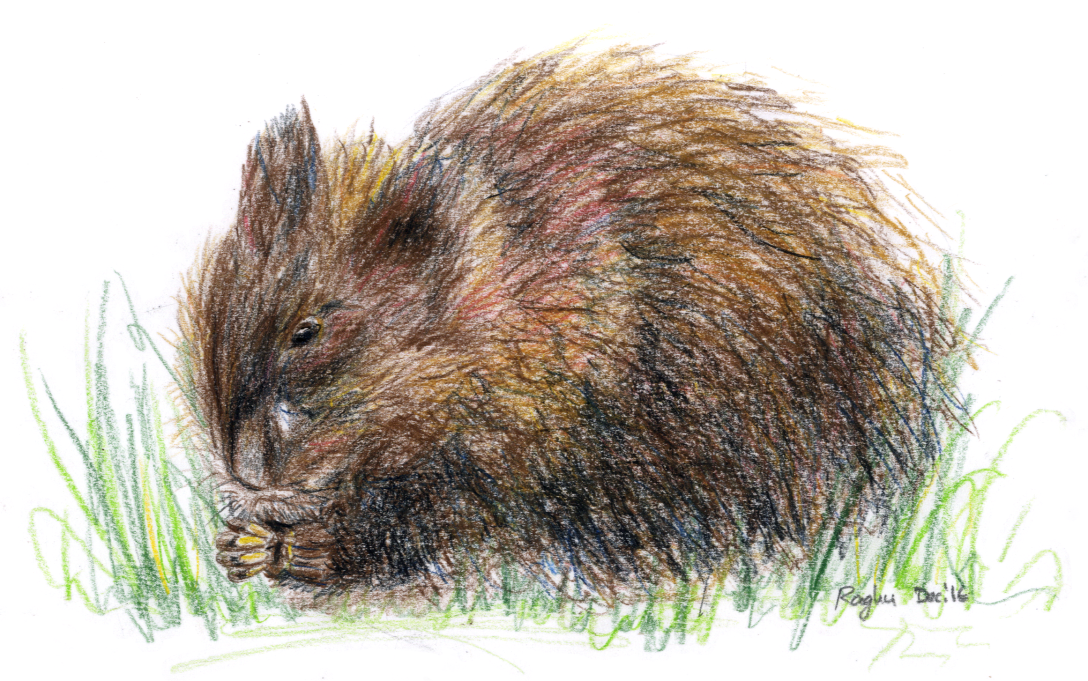
A muskrat, which I drew from this photo.