 In Part I, I wrote about how I started exploring the topic of machine learning, and we looked briefly described one of its main aims: automating the task of classifying objects based on their properties. Here, I’ll give an example of this in action, and also describe some general lessons I’ve drawn from this experience. The first part is probably not particularly interesting to most people, but it might help to make the ideas of Part I more concrete. The second part gets at the reasons I’ve found it rewarding to learn about machine learning, and why I think it’s a worthwhile activity for anyone in the sciences: the subject provides a neat framework for thinking about data, models, and what we can learn from the both of them.
1 I’d recognize that clump anywhere
I thought I’d create a somewhat realistic but simple example of applying machine learning to images, to be less abstract than the last post’s schematic of pears and bananas. My lab works with bacteria a lot, and a very common task in microbiology is to grow bacteria on agar plates and count the colonies to quantify bacterial abundance. (In case you want to make plates with your kids, by the way, check out [1].) Here’s what a plate with colonies looks like:
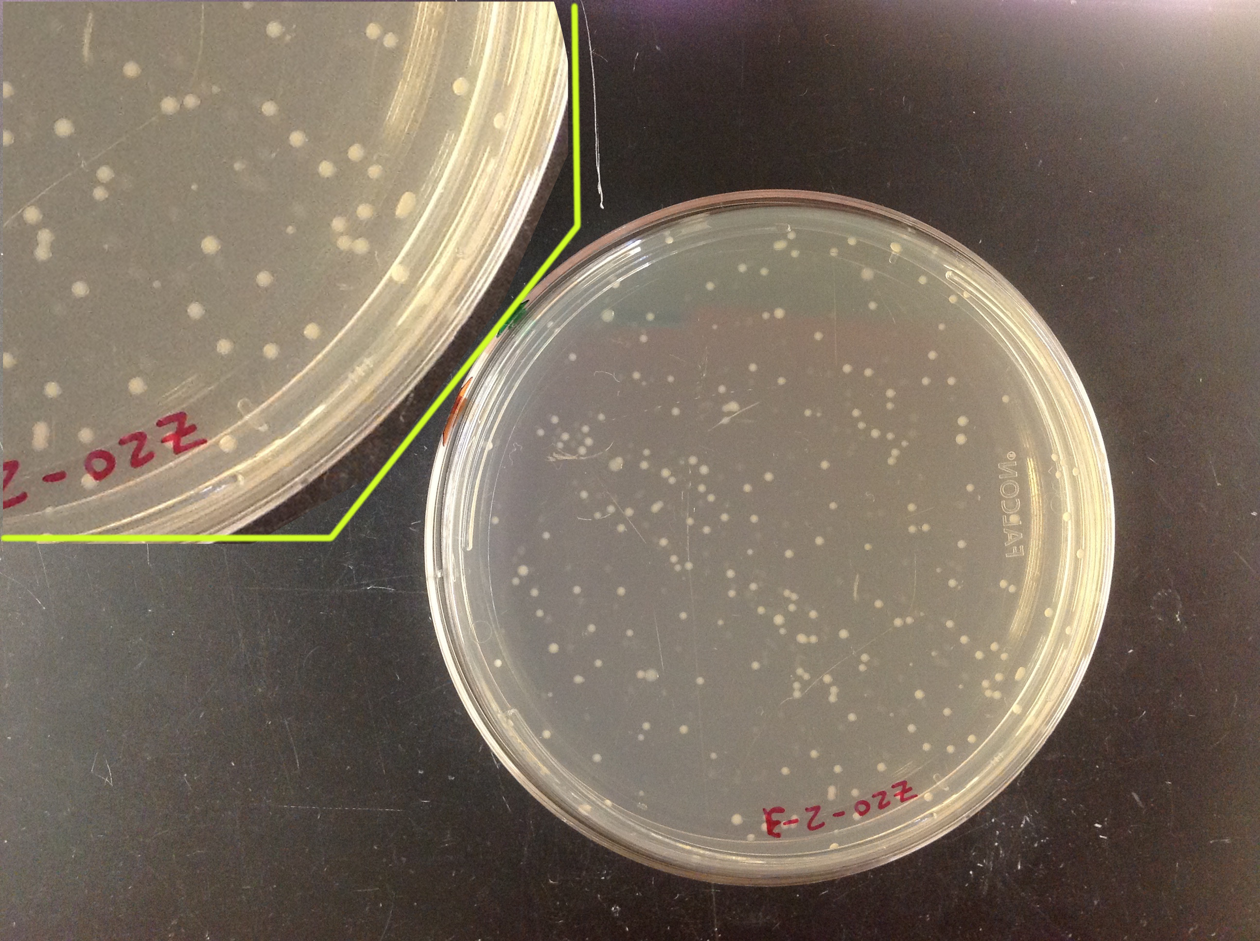 The colonies are the little white circles. Identifying them by eye is very easy. It’s also quite easy to write a non-machine-learning program to select the colonies, defining a priori thresholds for intensity and shape that distinguish colonies quite accurately. (In fact, I’ve assigned this as an exercise in an informal image analysis I’ve taught.) But, for kicks, let’s imagine we aren’t clever enough to think of a classification ourselves. How could we use machine learning?
1.1 Manual training
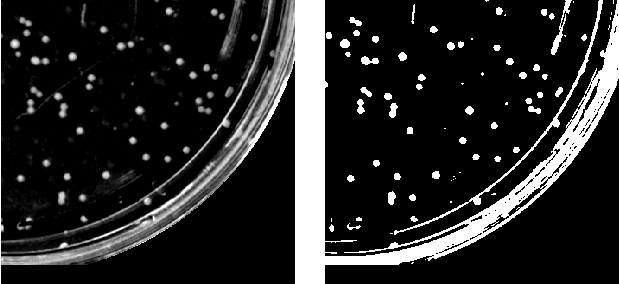
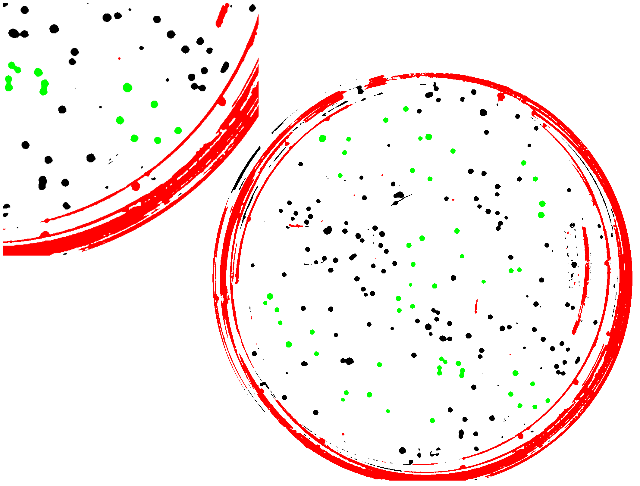
We first need to identify objects — colonies and things that aren’t colonies, like streaks of glare. Let’s do this by simple intensity thresholding, considering every connected set of pixels that are above some intensity threshold as an object. (Actually, I first identify the circle of the petri dish, and apply high- and low-pass filters, but this isn’t very interesting. I’ll comment more on this later.)
Next we create our “training set” — manually identifying some objects as being colonies, and some as not being colonies. I picked about 30 of each. The non-colonies tend to be large and elongated, or very small specks:
For each object, whether or not it’s in the training set, we can measure various properties: size, aspect ratio, intensity, orientation, etc. Like the pear and banana example in Part I, we want to create a boundary in the space of these parameters that separates colonies and not-colonies. What parameters should we consider? Let’s look at the area of each object relative to the median area of colonies, and the aspect ratio of each object, since these seem reasonable for distinguishing our targets. You might be aghast here — we’re having to be at least a little clever to think of parameters that are likely to be useful. What happened to letting the machine do things? I’ll return to this point later, also.
For colonies and not-colonies, what do these parameters look like? Let’s plot them — since I’ve chosen only two parameters, we can conveniently make a two-dimensional plot.
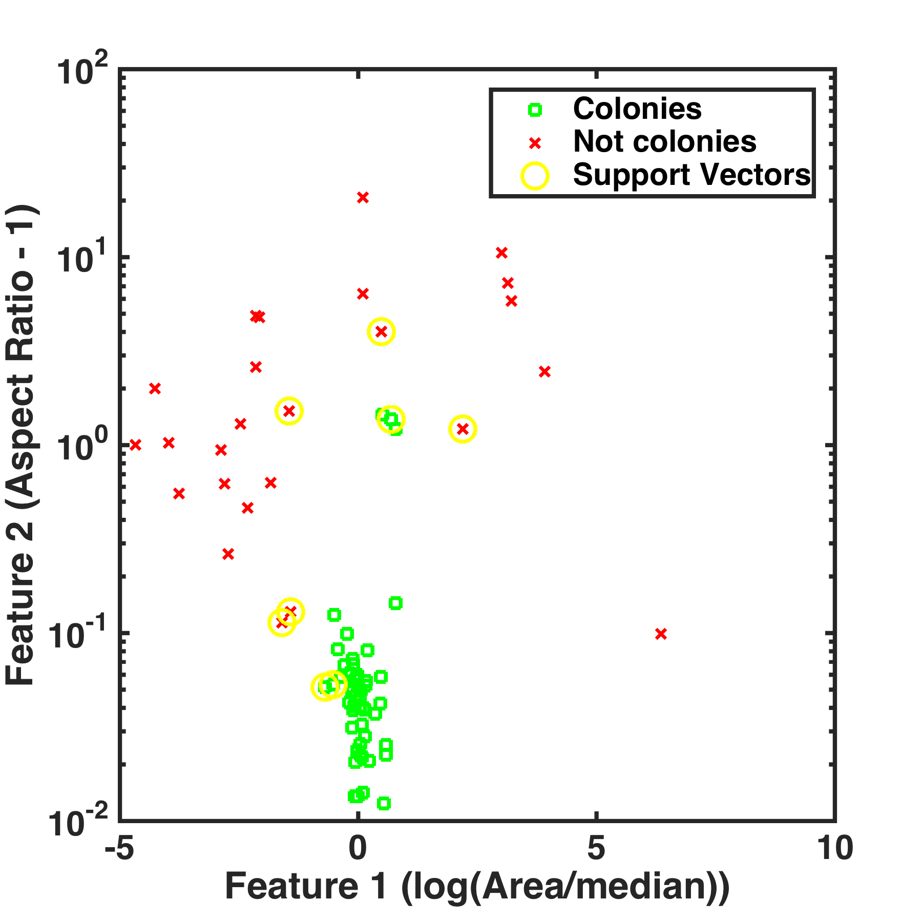 It does seem like we should be able to draw a boundary between these two classes. We’d like the optimal boundary, that maximizes the gap between the two classes, since this should give us the greatest accuracy in classifying future objects. Put differently, we not only want a boundary that separates colonies from non-colonies, but we want the thickest boundary such that colonies are on one side and non-colonies on the other. Technically, we want to maximize the “margin” between the two groups. A straight-line boundary is fairly straightforward to calculate, but it’s obvious that such a boundary won’t work here. Instead, we can try to transform the parameter space such that in the new space we can aim for a linear separation. One might imagine, perhaps, that instead of area and aspect ratio, the coordinates in the new space are area^3 and (aspect ratio)^2*area^4, for example. Remarkably, one doesn’t actually need to know the transformation from the normal parameter space; all we need is the inner product of vectors in this space. This approach, of determining optimal boundaries in some sort of parameter space, is that of a support vector machine, one of the key methods of machine learning. The actual calculation of the “support vectors,” the data points that lie on the optimal margin between the two groups, is a neat exercise in linear algebra and numerical optimization. The support vectors for our “training set” of manually-curated groups in the bacteria plate image are indicated by the yellow circles above.
There is, as one might guess, a great deal of flexibility in the choice of transformations. There is also freedom in setting the cost one assigns to objects of one class that lie in the territory of the other class. (In general it may be impossible to perfectly separate classes — imagine forcing a linear boundary on the training data above — so setting this cost is important.)
1.2 Does it work?
Now we’ve got a classifier — the “machine” has learned, from the data, a criterion for identifying colonies! I had to specify what parameters were relevant, and a few other things, but I never had to set anything about what values of these parameters differentiate colonies from non-colonies. We can now apply this classifier to new data, such a completely new plate image, using the same support vectors we just learned. If all has gone well, the algorithm will do a decent job of identifying what is and isn’t a colony. Let’s see:
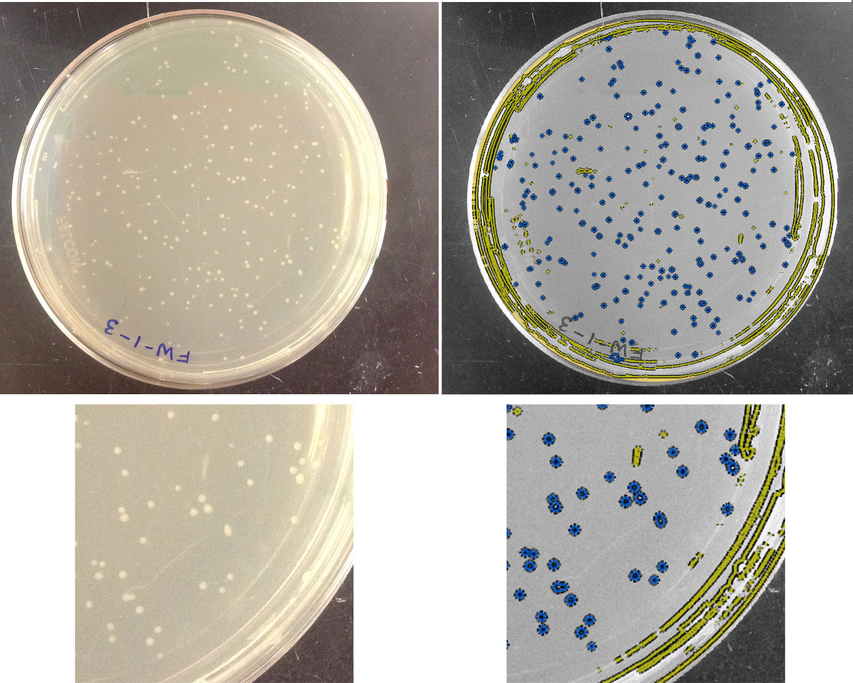
Not perfect, but pretty good! We could improve this with a larger set of training data, and by considering more or different parameters (though this can be dangerous, as I’ll get to shortly). Here’s what the object features look like:
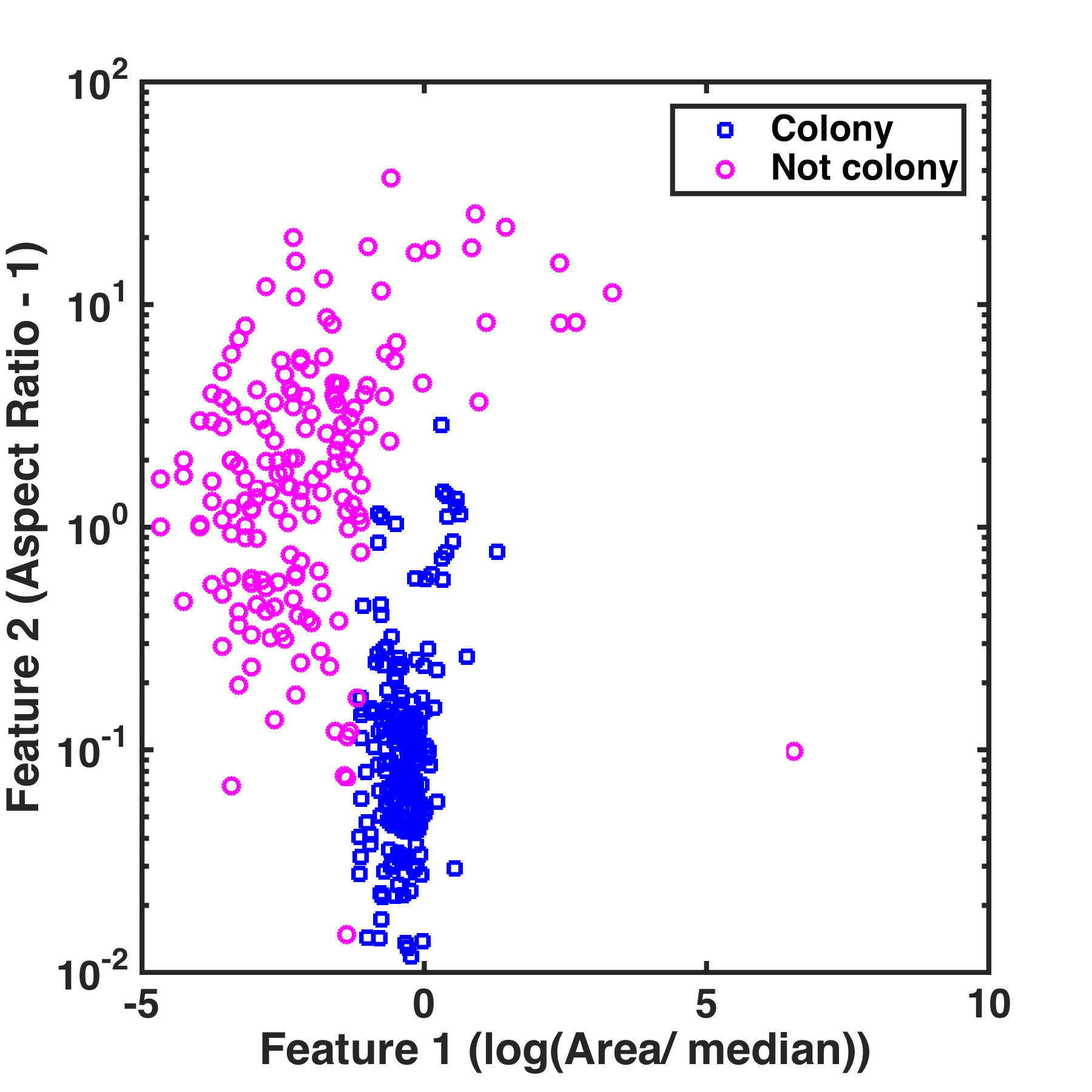 Again, it seems pretty good. There are probably a handful of mis-classified points. (I’m not going to bother actually figuring out the accuracy.)
So, there it is! Machine learning applied to bacterial colonies. If you look at the plates, you can see regions in which colonies have grown together, making two conjoined circles. We could go further and “learn” how to identify these pairs, again starting with a training set of manually identified objects. We could also iterate this process, finding errors in the machine classification and adding this to our training set. The possibilities are endless…
1.3 How sausage is made
Now let’s return to the several issues I glossed over. We first notice that we needed human input at several places, besides the creation of the training data set: identification of the plate, image filtering, choices of parameter transformations, etc. This seems rather non-machine-like. In principle, we could have learned all of these from the data as well: classifying pixels based as belonging to plate or non-plate, examining a space of possible filtering and other image manipulations, etc. However, each of these would have a substantial “cost” — a vast amount of training data on which to learn the appropriate classification. If we’re Google and have billions of annotated images on hand, this works; if not, it’s neither feasible nor appealing. Recall that we started using machine learning to avoid having to be “clever” about analysis algorithms. In practice, there’s a continuum of tradeoffs between how clever we need to be and how much data we’ve got.
We should be very careful, however. In general, we’ve got a lot of degrees of freedom at our disposal, and it would be easy to dangerously delude ourselves about the accuracy of our machine learning if we did not account for this flexibility. We could try, for example, lots of different “kernels” for transforming our parameter spaces; we may find that one works well — is this just by chance, or is it a robust feature of the sort of data we are considering? It’s especially troublesome that in general, the task of learning takes place in high-dimensional parameter spaces, not just the two-parameter space I used for this example, making it more difficult to visually determine whether things “make sense.”
2 Learning about data
Was learning about machine learning worthwhile?
From a directly practical point of view: yes. As mentioned at the start of the last post, my lab is already using approaches like those sketched above to extract information from complex images, and there’s lots of room for improvement. Especially if I view machine learning as an enhancement of human-driven analysis rather than an expectation that one’s algorithms act autonomously to make inferences from data, I can imagine many applications in my work. It has been rewarding to realize the continuum noted above that exists between human insight / little data and automation / lots of data, and it’s been good to learn some computational tools to use for this automation [2].
But this adventure has also been worthwhile from a broader point of view. The subject of machine learning provides a useful framework for thinking about data and models. Those of us who have been schooled in quantitative data learn a lot of good heuristics — having lots of parameters in a model is bad, for example. As Fermi famously said, “With four parameters I can fit an elephant, and with five I can make him wiggle his trunk.” More formally, we can think of model fitting as having the ultimate goal of minimizing the error between our model and future measurements (e.g. the second, “test” plate above), but with the constraint that all we have access to are our present measurements (the “training” plate). It is, of course, easy to overfit the training data, giving a model that fits it perfectly but that fails badly on the future tests. This is both because we may be simply fitting to noise in the training data, and because fitting models that are overly complex expands the ways in which we can miss the unknowable, “true” process that describes the data, even in the absence of noise.
Much of the machine learning course dealt with the statistical tools to understand and deal with these sorts of issues — regularization to “dampen” parameters, cross-validation to break up training data into pieces to test on, etc. None of this is shocking, but I had never explored it systematically.
What was shocking, though, was to learn a bit of the more abstract concepts underlying machine learning, such as how to assess whether it is possible for algorithms to classify data, and how this feeds into bounds on classification error (e.g. this). It’s fascinating. It’s also fairly recent, dating in large part just a few decades into the past. I generally think I’m pretty well read in a variety of areas, but I really was unaware that much of this existed! It’s a great feeling to uncover something new and unexpected. That in itself would have made the course worthwhile!
3 Learning about Mega Man
Continuing the illustration theme of Part I, I drew Mega Man (at the top of the post), which took far more time than I should admit to. K. did a quick sketch:
 [1] The present issue of Cultures, from the American Society for Microbiology, is the “Kid’s Issue.” Click here for the PDF and here for the “Flipbook.” Pages 96-97 describe how to make your own gel in which to grow cultures.
[2] I’ve written everything I’ve done, both for the course and these examples, in MATLAB, using the LIBSVM library [https://www.csie.ntu.edu.tw/~cjlin/libsvm/]. For one homework assignment, I wrote my own support vector machine algorithm, which made me realize how wonderfully fast LIBSVM is.
